Variable Importance in Random Forests

Predictive vs. interpretational overfitting

There appears to be broad consenus that random forests rarely suffer from “overfitting” which plagues many other models. (We define overfitting as choosing a model flexibility which is too high for the data generating process at hand resulting in non-optimal performance on an independent test set.) By averaging many (hundreds) of separately grown deep trees -each of which inevitably overfits the data – one often achieves a favorable balance in the bias variance tradeoff.
For similar reasons, the need for careful parameter tuning also seems less essential than in other models.

This post does not attempt to contribute to this long standing discussion (see e.g. https://stats.stackexchange.com/questions/66543/random-forest-is-overfitting) but points out that random forests’ immunity to overfitting is restricted to the predictions only and not to the default variable importance measure!

We assume the reader is familiar with the basic construction of random forests which are averages of large numbers of individually grown regression/classification trees. The random nature stems from both “row and column subsampling’’: each tree is based on a random subset of the observations, and each split is based on a random subset of candidate variables. The tuning parameter – which for popular software implementations has the default \(\lfloor p/3 \rfloor\) for regression and \(\sqrt{p}\) for classification trees – can have profound effects on prediction quality as well as the variable importance measures outlined below.

At the heart of the random forest library is the CART algorithm which chooses the split for each node such that maximum reduction in overall node impurity is achieved. Due to the CART bootstrap row sampling, \(36.8\%\) of the observations are (on average) not used for an individual tree; those “out of bag” (OOB) samples can serve as a validation set to estimate the test error, e.g.:
\[\begin{equation}
E\left( Y – \hat{Y}\right)^2 \approx OOB_{MSE} = \frac{1}{n} \sum_{i=1}^n{\left( y_i – \overline{\hat{y}}_{i, OOB}\right)^2}
\end{equation}\]

where \(\overline{\hat{y}}_{i, OOB}\) is the average prediction for the \(i\)th observation from those trees for which this observation was OOB.

Variable Importance

The default method to compute variable importance is the mean decrease in impurity (or gini importance) mechanism: At each split in each tree, the improvement in the split-criterion is the importance measure attributed to the splitting variable, and is accumulated over all the trees in the forest separately for each variable. Note that this measure is quite like the \(R^2\) in regression on the training set.

The widely used alternative as a measure of variable importance or short permutation importance is defined as follows:
\[\begin{equation}
\label{eq:VI}
\mbox{VI} = OOB_{MSE, perm} – OOB_{MSE}
\end{equation}\]

(more pointers in https://stackoverflow.com/questions/15810339/how-are-feature-importances-in-randomforestclassifier-determined)

Gini importance can be highly misleading

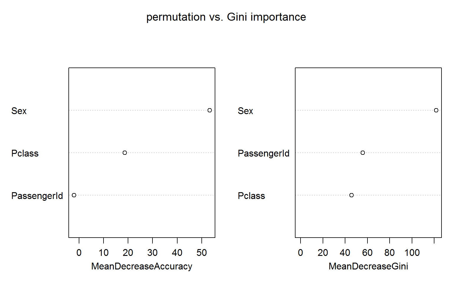
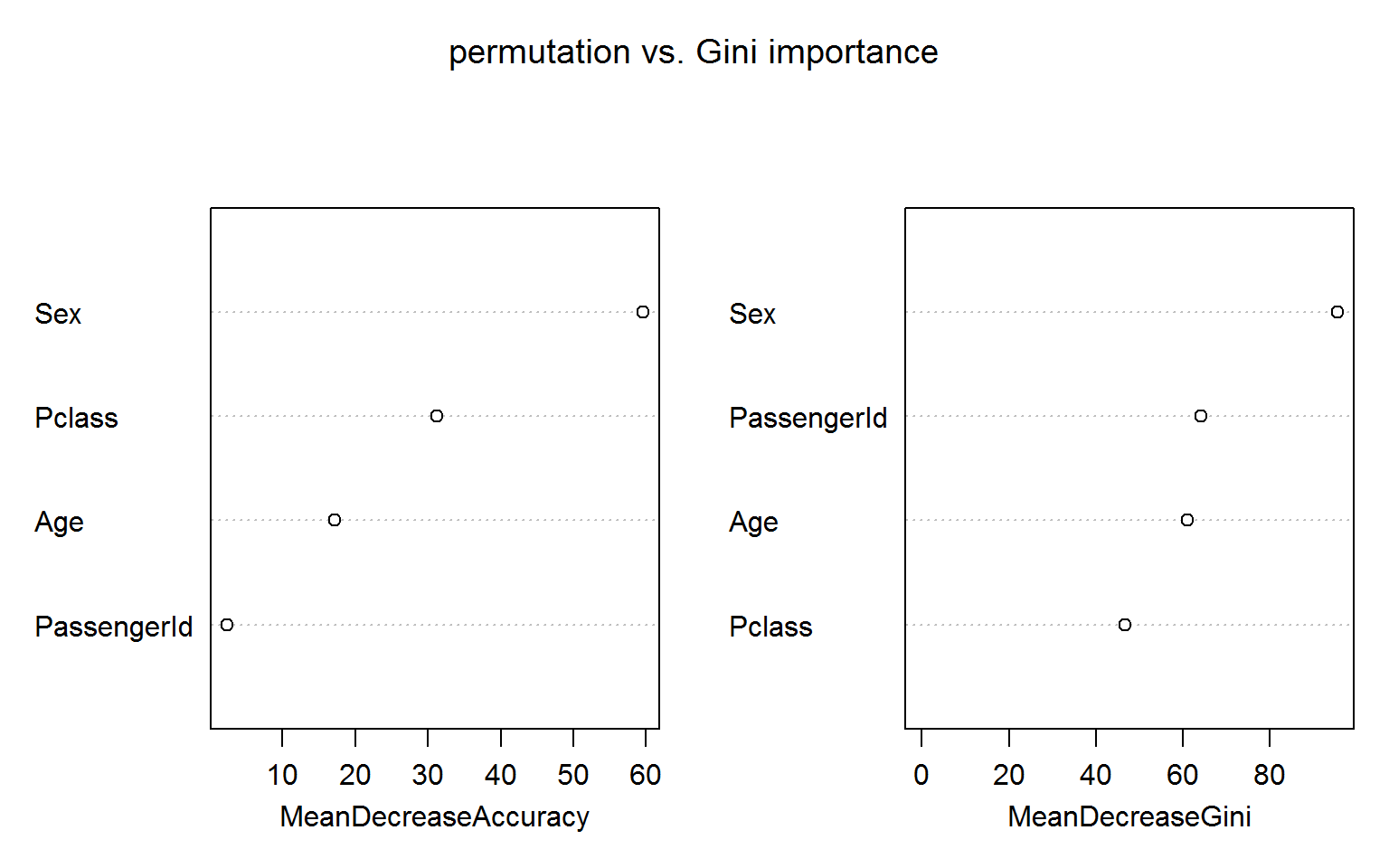
We use the well known titanic data set to illustrate the perils of putting too much faith into the Gini importance which is based entirely on training data – not on OOB samples – and makes no attempt to discount impurity decreases in deep trees that are pretty much frivolous and will not survive in a validation set.

In the following model we include passengerID as a feature along with the more reasonable Age, Sex and Pclass: randomForest(Survived ~ Age + Sex + Pclass + PassengerId, data=titanic_train[!naRows,], ntree=200,importance=TRUE,mtry=2)

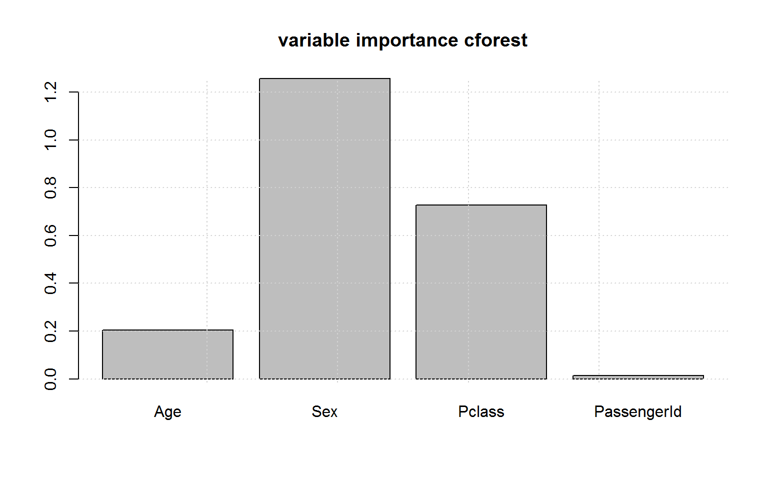
The figure below shows both measures of variable importance and surprisingly passengerID turns out to be ranked number 2 for the Gini importance (right panel). This unexpected result is robust to random shuffling of the ID.

The permutation based importance (left panel) is not fooled by the irrelevant ID feature. This is maybe not unexpected as the IDs shold bear no predictive power for the out-of-bag samples.

Noise Feature

Let us go one step further and add a Gaussian noise feature, which we call PassengerWeight:

titanic_train$PassengerWeight = rnorm(nrow(titanic_train),70,20)
rf4 =randomForest(Survived ~ Age + Sex + Pclass + PassengerId + PassengerWeight, data=titanic_train[!naRows,], ntree=200,importance=TRUE,mtry=2)

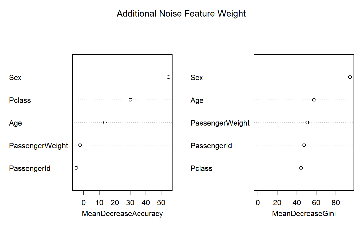
Again, the blatant “overfitting” of the Gini variable importance is troubling whereas the permutation based importance (left panel) is not fooled by the irrelevant features. (Encouragingly, the importance measures for ID and weight are even negative!)

In the remainder we investigate if other libraries suffer from similar spurious variable importance measures.
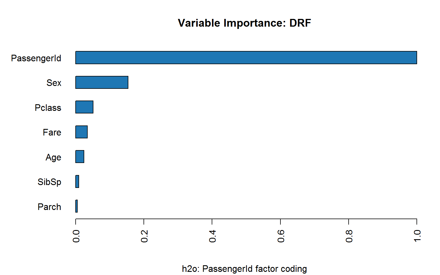
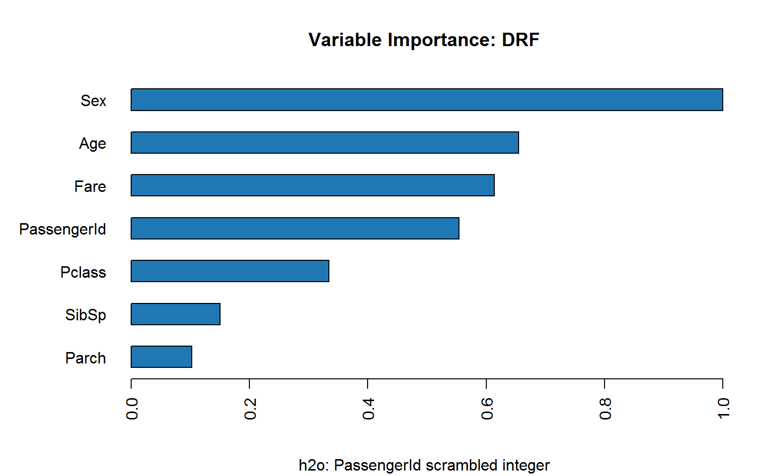
h2o library

Unfortunately, the h2o random forest implementation does not offer permutation importance:

https://stackoverflow.com/questions/51584970/permutation-importance-in-h2o-random-forest/51598742#51598742

Coding passenger ID as integer is bad enough:

Coding passenger ID as factor makes matters worse:

Let’s look at a single tree from the forest:

If we scramble ID, does it hold up?

partykit

conditional inference trees are not being fooled by ID:

And the variable importance in cforest is indeed unbiased

python’s sklearn

Unfortunately, like h2o the python random forest implementation offers only Gini importance, but this insightful post offers a solution:

http://explained.ai/rf-importance/index.html

Gradient Boosting

Boosting is highly robust against frivolous columns:

mdlGBM = gbm(Survived ~ Age + Sex + Pclass + PassengerId +PassengerWeight, data= titanic_train, n.trees = 300, shrinkage = 0.01, distribution = "gaussian")
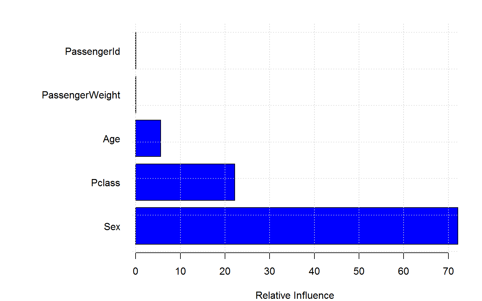
Conclusion

Sadly, this post is 12 years behind:

It has been known for while now that the Gini importance tends to inflate the importance of continuous or high-cardinality categorical variables:

the variable importance measures of Breiman’s original Random Forest method … are not reliable in situations where potential predictor variables vary in their scale of measurement or their number of categories.

(Strobl et al, 2007 Bias in random forest variable importance measures: Illustrations, sources and a solution)

Single Trees

I am still struggling with the extent of the overfitting. It is hard to believe that passenger ID could be chosen as a split point early in the tree building process given the other informative variables! Let us inspect a single tree

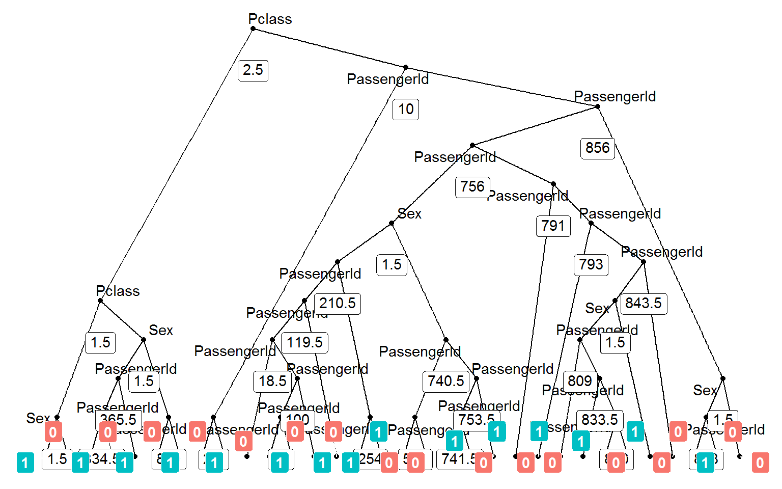
##   rowname left daughter right daughter   split var split point status
## 1       1             2              3      Pclass         2.5      1
## 2       2             4              5      Pclass         1.5      1
## 3       3             6              7 PassengerId        10.0      1
## 4       4             8              9         Sex         1.5      1
## 5       5            10             11         Sex         1.5      1
## 6       6            12             13 PassengerId         2.5      1
##   prediction
## 1       <NA>
## 2       <NA>
## 3       <NA>
## 4       <NA>
## 5       <NA>
## 6       <NA>

This tree splits on passenger ID at the second level !! Let us dig deeper:

The help page states

For numerical predictors, data with values of the variable less than or equal to the splitting point go to the left daughter node.

So we have the 3rd class passengers on the right branch. Compare subsequent splits on (i) sex, (ii) Pclass and (iii) passengerID:

Starting with a parent node Gini impurity of 0.184

Splitting on sex yields a Gini impurity of 0.159

1 2
0 72 303
1 71 50

Splitting on passengerID yields a Gini impurity of 0.183

FALSE TRUE
0 2 373
1 3 118

And how could passenger ID accrue more importance than sex ?


Customizing map background in Tableau

Tableau Desktop includes a connection to Tableau’s map server, which provides an extensive selection of maps optimized for use with Tableau. If you prefer to use your own maps, the easiest approach is to connect to a map server that supports the WMS standard. For more information, go to Working with WMS Servers topic in Tableau Desktop Help and Mapping Data with WMS article.

Requirements for a TMS Connection

To connect to your map server from the TMS, your map server must have the following features:

  • Maps are returned as a collection of tiles
  • Tiles are in Web Mercator projection
  • Tiles can be addressed by URL using the same numbering scheme as common web mapping services. For more information, see the <url-format> section under Variables in the TMS File for more information.

Create a Simple TMS File

To connect to the TMS, you must create a TMS file. A TMS file is a simple text file that you can create in a text editor.

Open a text editor.Copy and paste the following XML into the text editor.

Copy and paste the following XML into the text editor.<?xml version="1.0" encoding="utf-8"?>
<mapsource inline="<boolean>" version="8.1">
<connection class="OpenStreetMap" port="80" server="<server-url>" url-format="<url-format>" />
<layers>
<layer display-name='Base' name='base' show-ui='false' type='features' request-string='/' />
</layers>
</mapsource>

Replace <boolean>, <server-url>, and <url-format> variables as described in the Required Variables in the TMS File section in this article.

Save the TMS file with a .tms extension to the Mapsources folder of Tableau Desktop or Tableau Server.The default location for the Mapsources folder:

For Tableau Desktop on the Mac – /Users/<user>/Documents/My Tableau Repository/Mapsources

For Tableau Desktop on Windows – C:\Users\<user>\Documents\My Tableau Repository\Mapsources

For Tableau Server – C:\Program Files\Tableau\Tableau Server\<version>\vizqlserver\mapsources

Open Tableau Desktop.

Connect to a workbook that contains location information.

Select Map > Background Maps, and then select the background map from the map server you configured in the TMS file.

(Optional) If you added the TMS file to the Mapsources folder in Tableau Server, publish the workbook to Tableau Server and see the background map you configured in the TMS file.

Required Variables in the TMS File

Only the following variables can be changed in the XML:

<boolean>: Replace the <boolean> with either a true or false value.

A true value allows Tableau Desktop to save the configuration specified in the TMS file with the workbook. Use this value if your workbook is being published to Tableau Online or Tableau Public.

A false value requires Tableau Desktop or Tableau Server to have access to the TMS file saved in the Mapsources folder to display the maps from your map server.

<server-url>: Replace <server-url> with the URL of your map server.

<url-format>: Replace <url-format> with additional URL fragments that your map server requires. This might include the following tags:

{Z}: The {Z} tag indicates the zoom level. A zoom level of 0 displays the entire world in one map tile. The TMS will fetch map tiles up to level 16.

{X} and {Y}: The {X} and {Y} tags indicate the map tile coordinates. For more information about map tiles, refer to the following web pages:

OpenStreetMaps wiki page

Bing Maps web page

OSM XML

Suppose you want to connect to a sample map server provided by OpenStreetMaps. The TMS file may look like the following:

<?xml version="1.0" encoding="utf-8"?>
<mapsource inline="true" version="8.1">
<connection class="OpenStreetMap" port="80" server="http://a.tile.openstreetmap.org" url-format="/{Z}/{X}/{Y}.png" />
<layers>
<layer display-name='Base' name='base' show-ui='false' type='features' request-string='/' />
</layers>
</mapsource>

Google maps XML

The TMS file for the google map tile server looks like the following:

<?xml version="1.0" encoding="utf-8"?>
<mapsource inline="true" version="8.1">
<connection class="OpenStreetMap" port="80" <connection class="OpenStreetMap" port="80" server="http://mt1.google.com" url-format="/vt/lyrs=m&amp;x={X}&amp;y={Y}&amp;z={Z}" />
<layers>
<layer display-name='Base' name='base' show-ui='false' type='features' request-string='/' />
</layers>
</mapsource>

Stamen Toner XML

Suppose you want to connect to a sample map server provided by OpenStreetMaps. The TMS file may look like the following:

<?xml version="1.0" encoding="utf-8"?>
<mapsource inline="true" version="8.1">
<connection class="OpenStreetMap" port="80" <connection class="OpenStreetMap" port="80"
server="http://tile.stamen.com" url-format="/toner/{Z}/{X}/{Y}.png" />
<layers>
<layer display-name='Base' name='base' show-ui='false' type='features' request-string='/' />
</layers>
</mapsource>

Stamen WaterColor XML

Suppose you want to connect to a sample map server provided by OpenStreetMaps. The TMS file may look like the following:

<?xml version="1.0" encoding="utf-8"?>
<mapsource inline="true" version="8.1">
<connection class="OpenStreetMap" port="80" <connection class="OpenStreetMap" port="80"
<connection class="OpenStreetMap" port="80" server="http://tile.stamen.com" url-format="/watercolor/{Z}/{X}/{Y}.jpg" />
<layers>
<layer display-name='Base' name='base' show-ui='false' type='features' request-string='/' />
</layers>
</mapsource>


Offline maps: local map tile server

As described previously (e.g. http://rgooglemaps.r-forge.r-project.org/OfflineMaps-RgoogleMaps-leaflets.html) we can use the RgoogleMaps package to (i) download map tiles and store them locally and (ii) launch a local Web server (in python or in R) to serve the map tiles to ANY mapping application.

To achieve this in Tableau, you would simply follow the instructions from the link above and then use e.g. this XML file:

<?xml version="1.0" encoding="utf-8"?>
<mapsource inline="true" version="8.1">
<connection class="OpenStreetMap" port="80" <connection class="OpenStreetMap" port="80"
<connection class="OpenStreetMap" port="80" server="
http:/localhost:8000" url-format="/mapTiles/watercolor/{Z}/{X}/{Y}.jpg" />
<layers>
<layer display-name='Base' name='base' show-ui='false' type='features' request-string='/' />
</layers>
</mapsource>

Offline Maps with RgoogleMaps and leaflets


Offline Maps with RgoogleMaps and leaflets


New version of RgoogleMaps now fetches map tiles

Until version 1.3.0 RgoogleMaps only downloaded static maps as provided by the static maps APIs from e.g. Google, bing and OSM. While there are numerous advantages to this strategy such as full access to the extensive feature list provided by those APIs, the limitations are also clear:

  1. unlikely reusability of previously stored static maps,
  2. limits on the maximum size of the map (640,640),
  3. and the requirement to be online.

Beginning with version 1.4.1 (which is now on CRAN ) , we added the functions GetMapTiles and PlotOnMapTiles which fetch individual map tiles and store them locally.

For example, if we wanted to fetch 20 tiles (in each direction) at zoom level 16 around Washington Square Park in Manhattan, we would simply run

library(RgoogleMaps)
(center=getGeoCode("Washington Square Park;NY"))
##       lat       lon 
##  40.73082 -73.99733
GetMapTiles(center, zoom=16,nTiles = c(20,20))

Note that the default server is taken to be openstreetmap and the default local directory “~/mapTiles/OSM”. We could have also passed the location string directly and saved several zoom levels at once (note the constant radius adaptation of the number of tiles):

for (zoom in 13:15)
  GetMapTiles("Washington Square Park;NY", zoom=zoom,nTiles = round(c(20,20)/(17-zoom)))

Before requesting new tiles, the function checks if that map tile exists already which avoids redundant downloads.

We can repeat the process with Google map tiles and plot them:

for (zoom in 13:16)
  GetMapTiles("Washington Square Park;NY", zoom=zoom,nTiles = round(c(20,20)/(17-zoom)),
              urlBase = "http://mt1.google.com/vt/lyrs=m", tileDir= "~/mapTiles/Google/")

#just get 3x3 tiles:

#mt= GetMapTiles(center = c(lat = 40.73082, lon =-73.99733), zoom=16,nTiles = c(3,3), urlBase = "http://mt1.google.com/vt/lyrs=m", tileDir= "~/mapTiles/Google/", returnTiles = TRUE)

mt= GetMapTiles("Washington Square Park;NY", zoom=16,nTiles = c(3,3),
              urlBase = "http://mt1.google.com/vt/lyrs=m", tileDir= "~/mapTiles/Google/", returnTiles = TRUE)
PlotOnMapTiles(mt)

unnamed-chunk-3-1

Interactive Web Maps with the JavaScript ‘Leaflet’ Library

While the original motivation of GetMapTiles was to enable offline creation of static maps within the package RgoogleMaps, combining this feature with the interactivity of the leaflet library leads to an effective offline maps version of leaflet!

We only need to replace the default server specified by the parameter urlTemplate by a local server obliging with the file naming scheme zoom_X_Y.png set by GetMapTiles Any simple local Web service will suffice, but the following two solutions work best for me

  1. (http://stackoverflow.com/questions/5050851/best-lightweight-web-server-only-static-content-for-windows) “To use Python as a simple web server just change your working directory to the folder with your static content and type python -m SimpleHTTPServer 8000, everything in the directory will be available at http:/localhost:8000/

  2. (https://github.com/yihui/servr) Use the R package servr: Rscript -e ‘servr::httd()’ -p8000

So assuming (i) successful execution of the map tileabove and (ii) the correct launch of the server (in the parent dirtectory of mapTiles/), the following code will have leaflet dynamically load them (from the local repository) for zooming and panning abilities:

library(leaflet)
  m = leaflet::leaflet() %>% 
    addTiles( urlTemplate = "http:/localhost:8000/mapTiles/OSM/{z}_{x}_{y}.png")
  m = m %>% leaflet::setView(-73.99733, 40.73082 , zoom = 16)
  m = m %>% leaflet::addMarkers(-73.99733, 40.73082 )
  m

And for google map tiles:

library(leaflet)
  m = leaflet::leaflet() %>% 
    addTiles( urlTemplate = "http:/localhost:8000/mapTiles/Google/{z}_{x}_{y}.png")
  m = m %>% leaflet::setView(-73.99733, 40.73082 , zoom = 16)
  m = m %>% leaflet::addMarkers(-73.99733, 40.73082 )
  m