Interpretation of the coefficients in logistic regression


Interpretation of the coefficients in logistic regression


Fitting a logistic regression (LR) model (with Age, Sex and Pclass as predictors) to the survival outcome in the Titanic data yields a summary such as this one:

## 
## Call:
## glm(formula = Survived ~ Age + Sex + Pclass, family = binomial(link = logit), 
##     data = NoMissingAge)
## 
## Deviance Residuals: 
##     Min       1Q   Median       3Q      Max  
## -2.7303  -0.6780  -0.3953   0.6485   2.4657  
## 
## Coefficients:
##              Estimate Std. Error z value Pr(>|z|)    
## (Intercept)  3.777013   0.401123   9.416  < 2e-16 ***
## Age         -0.036985   0.007656  -4.831 1.36e-06 ***
## Sexmale     -2.522781   0.207391 -12.164  < 2e-16 ***
## Pclass2     -1.309799   0.278066  -4.710 2.47e-06 ***
## Pclass3     -2.580625   0.281442  -9.169  < 2e-16 ***
## ---
## Signif. codes:  0 '***' 0.001 '**' 0.01 '*' 0.05 '.' 0.1 ' ' 1
## 
## (Dispersion parameter for binomial family taken to be 1)
## 
##     Null deviance: 964.52  on 713  degrees of freedom
## Residual deviance: 647.28  on 709  degrees of freedom
## AIC: 657.28
## 
## Number of Fisher Scoring iterations: 5
##          1          2          3          4          5          7 
## -0.4716467  0.4224490  1.0794775  0.4005642 -0.3747404 -0.8821915
##          1          2          3          4          5          7 
## -0.4716467  0.4224490  1.0794775  0.4005642 -0.3747404 -0.8821915

For “normal regression” we know that the value of \(\beta_j\) simply gives us \(\Delta y\) if \(x_j\) is increased by one unit.

In order to fully understand the exact meaning of the coefficients for a LR model we need to first warm up to the definition of a link function and the concept of probability odds.

Using linear regression as a starting point \[
y_i = \beta_0 + \beta_1 x_{1,i} + \beta_2 x_{2,i} + \ldots +\beta_k x_{k,i} + \epsilon_i
\]
we modify the right hand side such that (i) the model is still basically a linear combination of the \(x_j\)s but (ii) the output is -like a probability- bounded between 0 and 1. This is achieved by “wrapping” a sigmoid function \(s(z) = 1/(1+exp(z))\) around the weighted sum of the \(x_j\)s: \[
y_i = s(\beta_0 + \beta_1 x_{1,i} + \beta_2 x_{2,i} + \ldots +\beta_k x_{k,i} + \epsilon_i)
\]
The sigmoid function, depicted below to the left, transforms the real axis to the interval \((0;1)\) and can be interpreted as a probability.

The inverse of the sigmoid is the logit (depicted above to the right), which is defined as \(log(p/(1-p))\). For the case where p is a probability we call the ratio \(p/(1-p)\) the probability odds. Thus, the logit is the log of the odds and logistic regression models these log-odds as a linear combination of the values of x.

Finally, we can interpret the coefficients directly: the odds of a positive outcome are multiplied by a factor of \(exp(\beta_j)\) for every unit change in \(x_j\). (In that light, logistic regression is reminiscient of linear regression with logarithmically transformed dependent variable which also leads to multiplicative rather than additive effects.)

As an example, the coefficient for Pclass 3 is -2.5806, which means that the odds of survival compared to the reference level Pclass 1 are reduced by a factor of \(exp(-2.5806) = 0.0757\);with all other input variables unchanged. How does the relative change in odds translate into probabilities? It is relatively easy to memorize the to and forth relationship between odds and probability \(p\): \[
odds = \frac{p}{1-p} \Leftrightarrow p = \frac{odds}{1 + odds}
\]
So the intercept 3.777 (= log-odds!) translates into odds of \(exp(3.777) = 43.685\) which yields a base probability of survival (for female Pclass1 of age 0) of \(43.685/(1 + 43.685) = 0.978\)

Why make life so complicated?

I am often asked by students why we have to go through the constant trouble of (i) exponentiating the coefficients, (ii) multiplying the odds and finally (iii) compute the resulting probabilities? Can we not simply transform the coefficients from the summary table such that we can read off their effects directly – just like in linear regression?

The trouble is that there is no simple way to translate the coefficients into an additive or even a multiplicative adjustment of the probabilities. (One simple way to see this is the impossibility of keeping the output bounded between 0 and 1) The following graph shows the effect of various coefficient values on a base/reference probability.

We immediately see that there is no straightforward additive or multiplicative effect that could be quantified.


Is logistic regression resistant to outliers?


Is logistic regression resistant to outliers?


We speculate that the S-shaped sigmoid function is forgiving of outliers in x as long as one is “on the right side”, i.e. if the class label does not contradict the general trend of the variable. For example, in the Titanic data we have seen that survival probability tended to decline with increasing age. What if we added a \(500\)-year old person to the data set who did not survive? For linear regression such an outlier would likely distort the coefficient estimates significantly.

fit = glm(Survived ~ Age , data= NoMissingAge, family = binomial(link=logit))
summary(fit)
## 
## Call:
## glm(formula = Survived ~ Age, family = binomial(link = logit), 
##     data = NoMissingAge)
## 
## Deviance Residuals: 
##     Min       1Q   Median       3Q      Max  
## -1.1488  -1.0361  -0.9544   1.3159   1.5908  
## 
## Coefficients:
##             Estimate Std. Error z value Pr(>|z|)  
## (Intercept) -0.05672    0.17358  -0.327   0.7438  
## Age         -0.01096    0.00533  -2.057   0.0397 *
## ---
## Signif. codes:  0 '***' 0.001 '**' 0.01 '*' 0.05 '.' 0.1 ' ' 1
## 
## (Dispersion parameter for binomial family taken to be 1)
## 
##     Null deviance: 964.52  on 713  degrees of freedom
## Residual deviance: 960.23  on 712  degrees of freedom
## AIC: 964.23
## 
## Number of Fisher Scoring iterations: 4
dataWithOutlier = NoMissingAge
dataWithOutlier[1,c("Age", "Survived")] = c(500,0) 
fit = glm(Survived ~ Age , data= dataWithOutlier, family = binomial(link=logit))
summary(fit)
## 
## Call:
## glm(formula = Survived ~ Age, family = binomial(link = logit), 
##     data = dataWithOutlier)
## 
## Deviance Residuals: 
##     Min       1Q   Median       3Q      Max  
## -1.1515  -1.0373  -0.9545   1.3145   1.5928  
## 
## Coefficients:
##              Estimate Std. Error z value Pr(>|z|)  
## (Intercept) -0.050245   0.172124  -0.292   0.7704  
## Age         -0.011100   0.005271  -2.106   0.0352 *
## ---
## Signif. codes:  0 '***' 0.001 '**' 0.01 '*' 0.05 '.' 0.1 ' ' 1
## 
## (Dispersion parameter for binomial family taken to be 1)
## 
##     Null deviance: 964.52  on 713  degrees of freedom
## Residual deviance: 959.12  on 712  degrees of freedom
## AIC: 963.12
## 
## Number of Fisher Scoring iterations: 4
#what do the diagnostic plots tell us?
#plot(fit)
#and now we change the label which leads to a large residual:
dataWithOutlier[1,"Survived"] = 1 
fit = glm(Survived ~ Age , data= dataWithOutlier, family = binomial(link=logit))
summary(fit)
## 
## Call:
## glm(formula = Survived ~ Age, family = binomial(link = logit), 
##     data = dataWithOutlier)
## 
## Deviance Residuals: 
##    Min      1Q  Median      3Q     Max  
## -1.039  -1.026  -1.015   1.336   1.631  
## 
## Coefficients:
##              Estimate Std. Error z value Pr(>|z|)  
## (Intercept) -0.332154   0.131543  -2.525   0.0116 *
## Age         -0.001383   0.003553  -0.389   0.6970  
## ---
## Signif. codes:  0 '***' 0.001 '**' 0.01 '*' 0.05 '.' 0.1 ' ' 1
## 
## (Dispersion parameter for binomial family taken to be 1)
## 
##     Null deviance: 965.27  on 713  degrees of freedom
## Residual deviance: 965.11  on 712  degrees of freedom
## AIC: 969.11
## 
## Number of Fisher Scoring iterations: 4

Wow, one data point changes the entire fit significantly in the second case but left it virtually alone in the first.


kaggle@HWR

“Kaggling” at HWR has been used as a successful teaching tool since Fall 2014 when the first batch of “Business Intelligence and Process Management” (BIPM) master students embarked upon 2 competitions in the course Learning from structured Data taught by Prof. Loecher.

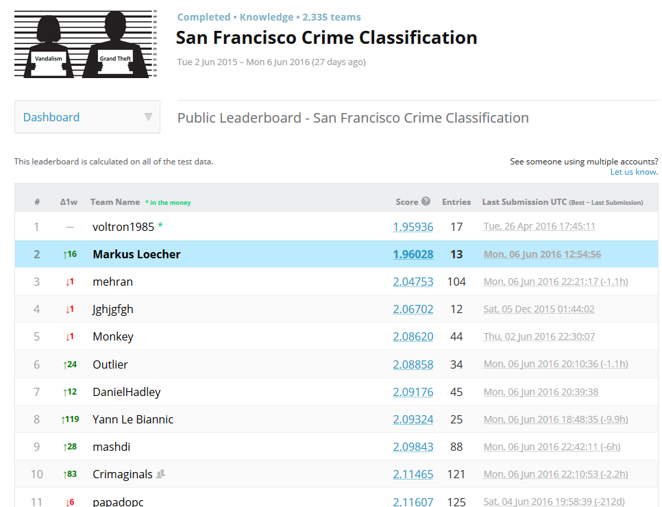
While the participation was never meant to be a serious attempt at competing with the many hard working and highly talented teams in the world, we are proud to announce that we actually made the top 10 in the San Francisco Crime Classification leaderboard, yeah!

kaggle_SFCrime_SubmissionTop10

UPDATE: The competition is officially over, and we are very happy to announce that we ended up in 2nd place:

kaggle_SFCrime_SubmissionTop2